Difference between Beta + Binomial vs. BetaBinomal (Statistical Rethinking example)

[rbudnar]

Hi! A bit of a beginner question here. I’m working through some examples in Statistical Rethinking and I am having trouble understanding what is happening differently when using the BetaBinomial distribution directly vs. parameterizing a Binomial distribution with a beta distribution. The example is the admissions data with gender from chapter 12 (Mixture models) and the notebook I worked from is here.

The original version with BetaBinomial is this:

# Code 12.2
UCBadmit = pd.read_csv("../data/UCBadmit.csv", sep=";")
d = UCBadmit
d["gid"] = (d["applicant.gender"] != "male").astype(int)


dat = dict(A=d.admit.values, N=d.applications.values, gid=d.gid.values)

def model(gid, N, A=None):
    a = numpyro.sample("a", dist.Normal(0, 1.5).expand([2]))
    phi = numpyro.sample("phi", dist.Exponential(1))
    theta = numpyro.deterministic("theta", phi + 2)
    pbar = expit(a[gid])
    numpyro.sample("A", dist.BetaBinomial(pbar * theta, (1 - pbar) * theta, total_count=N), obs=A)


m12_1 = MCMC(NUTS(model), num_warmup=500, num_samples=500, num_chains=4)
m12_1.run(random.PRNGKey(0), **dat)

I wanted to see what would happen when breaking it down into Beta + Binomial; the only thing that changed was the last two lines of the model where I added the p and then used the Binomial directly.

dat = dict(A=d.admit.values, N=d.applications.values, gid=d.gid.values)

def model_1a(gid, N, A=None):
    a = numpyro.sample("a", dist.Normal(0, 1.5).expand([2]))
    phi = numpyro.sample("phi", dist.Exponential(1))
    theta = numpyro.deterministic("theta", phi + 2)
    pbar = expit(a[gid])
    p = numpyro.sample("p", dist.Beta(pbar * theta, (1 - pbar) * theta))
    numpyro.sample("A", dist.Binomial(total_count=N, probs=p), obs=A)


m12_1a = MCMC(NUTS(model_1a), num_warmup=500, num_samples=500, num_chains=4)
m12_1a.run(random.PRNGKey(0), **dat)

The print_summary results are pretty close to the same for both models (though there’s now values for p in the second).

# Code 12.3 - original verison
post = m12_1.get_samples()
post["theta"] = Predictive(m12_1.sampler.model, post)(random.PRNGKey(1), **dat)["theta"]
post["da"] = post["a"][:, 0] - post["a"][:, 1]
print_summary(post, 0.89, False)

# Updated version with beta + binomial
post_1a = m12_1a.get_samples()
post_1a["theta"] = Predictive(m12_1a.sampler.model, post_1a)(random.PRNGKey(1), **dat)["theta"]
post_1a["da"] = post_1a["a"][:, 0] - post_1a["a"][:, 1]
print_summary(post_1a, 0.89, False)

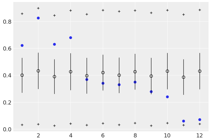
However, when doing the posterior predictive checks, the second model essentially predicts the empirical data:

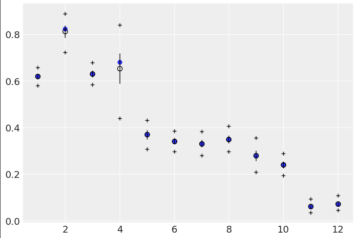
Code for above:

# Code 12.5
post = m12_1a.get_samples()
admit_pred = Predictive(m12_1a.sampler.model, post_1a)(
    random.PRNGKey(1), gid=dat["gid"], N=dat["N"]
)["A"]
admit_rate = admit_pred / dat["N"]
plt.scatter(range(1, 13), dat["A"] / dat["N"])
plt.errorbar(
    range(1, 13),
    jnp.mean(admit_rate, 0),
    jnp.std(admit_rate, 0) / 2,
    fmt="o",
    c="k",
    mfc="none",
    ms=7,
    elinewidth=1,
)
plt.plot(range(1, 13), jnp.percentile(admit_rate, 5.5, 0), "k+")
plt.plot(range(1, 13), jnp.percentile(admit_rate, 94.5, 0), "k+")
plt.show()

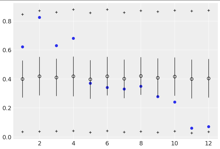
For reference, here’s the first model (code 12.5):

I peeked under the hood of the code for BetaBinomial and it appears to be creating a Beta distribution and sampling from it, then feeding those probs to a Binomial distribution - in other words it seems like it is doing the same thing I thought I was doing by splitting it apart.

Can anyone help me understand why there’s difference in the predicted values in this case? I think the results of the Beta + Binomial make more sense to me than the BetaBinomial, but I’m not sure how to interrogate the results to spot why it is different. Is there some kind of pooling effect happening with BetaBinomial?

Thanks, and sorry for the long post!
Ron

[fritzo]

The difference is that the p in the first model is local to each observation (i.e. there are many ps) whereas in the second model there is a single global p that fits all the data. If you had put your p statement inside a plate, then the results should be similar:

def model_2(gid, N, A=None):
    a = numpyro.sample("a", dist.Normal(0, 1.5).expand([2]))
    phi = numpyro.sample("phi", dist.Exponential(1))
    theta = numpyro.deterministic("theta", phi + 2)
    pbar = expit(a[gid])
    with numpyro.plate("data", len(A)):
        p = numpyro.sample("p", dist.Beta(pbar * theta, (1 - pbar) * theta))
        numpyro.sample("A", dist.Binomial(total_count=N, probs=p), obs=A)

It’s probably safer to explicitly declare your plates, e.g. I would have written

def model_1a(gid, N, A=None):
    a = numpyro.sample("a", dist.Normal(0, 1.5).expand([2]))
    phi = numpyro.sample("phi", dist.Exponential(1))
    theta = numpyro.deterministic("theta", phi + 2)
    pbar = expit(a[gid])
    p = numpyro.sample("p", dist.Beta(pbar * theta, (1 - pbar) * theta))
    with numpyro.plate("data", len(A)):
        numpyro.sample("A", dist.Binomial(total_count=N, probs=p), obs=A)

You can then visualize the difference between the models using render_model().

[rbudnar]

Thanks! I might be misunderstanding, but the non-plated version I posted already has many ps. I believe this is due to how pbar is constructed by indexing the a variable (the shape of pbar is (12,).) Here’s the print summary from the second model I posted:

                mean       std    median      5.5%     94.5%     n_eff     r_hat
      a[0]     -0.44      0.41     -0.45     -1.09      0.17   2629.70      1.00
      a[1]     -0.33      0.43     -0.34     -1.03      0.34   2341.87      1.00
      p[0]      0.62      0.02      0.62      0.59      0.65   3022.45      1.00
      p[1]      0.81      0.04      0.81      0.75      0.87   2678.93      1.00
      p[2]      0.63      0.02      0.63      0.60      0.66   3792.28      1.00
      p[3]      0.65      0.09      0.66      0.53      0.81   3768.06      1.00
      p[4]      0.37      0.03      0.37      0.32      0.41   3646.33      1.00
      p[5]      0.34      0.02      0.34      0.31      0.37   2956.96      1.00
      p[6]      0.33      0.02      0.33      0.29      0.37   2967.18      1.00
      p[7]      0.35      0.03      0.35      0.31      0.39   3672.46      1.00
      p[8]      0.28      0.03      0.28      0.22      0.33   2725.74      1.00
      p[9]      0.24      0.02      0.24      0.21      0.27   2874.80      1.00
     p[10]      0.06      0.01      0.06      0.04      0.08   2753.77      1.00
     p[11]      0.07      0.01      0.07      0.05      0.10   3032.76      1.00
       phi      1.04      0.80      0.86      0.01      2.09   2532.06      1.00

I added in the plate in both ways you showed above, but the print_summary output was identical. If I remove the indexing of a by gid and then use a plate on just the observed A, I then get a single p.

[fritzo]

Hmm not sure then, maybe @fehiepsi understands what’s going on?

[fehiepsi]

In the second model, you learned posterior for each p and then use it for each point prediction. In the first model, you generate p from a Beta distribution. Two approaches are different. If you remove the posterior samples of p after doing MCMC, you might get similar results. Getting posterior for each p gives you the sense of the probability of each Binomial observation, but if you want to apply the model and posterior samples for new dataset, you need to remove p posterior samples to make predictions.

A similar scenario is you build a generative model p(X,z). In the first model, you get posterior samples p(z|X) then use those samples to simulate the model, you will get what we called posterior predictive. Similar to the second model, you can also get posterior samples p(z, X|X), then if you use those samples for posterior predictive, you will get all X.

[rbudnar]

@fehiepsi

In the second model, you learned posterior for each p and then use it for each point prediction. In the first model, you generate p from a Beta distribution

Conceptually, I think that makes sense to me. In the second model, there are separately learned posteriors for p. It sounds like there’s only a single p in the case of the first model?

In practice, I think I’m confused since both models end up with 12 different pbars (really 2 since there are 2 gids) parameterizing their Beta distributions since they both have expit(a[gid]). I was looking at the source code for BetaBinomial, and I see it sampling probabilities from its underlying beta. From what I can tell, both the beta distributions from the first and second model are getting the same shape, which in this case would be (12,). If that’s the case, what happens to make it such that there’s only a single p? Or is that not really what’s happening?

Maybe another way to phrase this would be - is it possible to rewrite the second model in such a way that reproduces the first model (still using a separate beta distribution)? It sounds like this is what you were getting at with this statement: If you remove the posterior samples of p after doing MCMC, you might get similar results.

Thanks again!

[fehiepsi]

While simulating the model, p will be drawn from a Beta distribution with mean pbar (which has shape 12). Could you print out the summary of the posterior for a? If posterior of expit(a[0]) is similar to expit(a[1]), then the plot is expected because those 12 different Beta has similar parameters. For both models, the latent p will have shape 12. Because pbar has shape 12, I’m not sure how to construct a similar model with just 1 p (maybe taking average of pbar? - that creates a different model)

is it possible to rewrite the second model in such a way that reproduces the first model

That’s right. You can remove posterior samples of p to get similar predictive distributions.

[rbudnar]

@fehiepsi

You can remove posterior samples of p to get similar predictive distributions.

Ok I was definitely overthinking this at first. It was just this:

post = m12_1a.get_samples()
post = { key: value for key, value in post.items() if key != "p"}

and as you said, that resulted in a similar chart to the original model:

The summary from that looks like this:

               mean       std    median      5.5%     94.5%     n_eff     r_hat
      a[0]     -0.44      0.41     -0.45     -1.09      0.17   2629.70      1.00
      a[1]     -0.33      0.43     -0.34     -1.03      0.34   2341.87      1.00
      p[0]      0.62      0.02      0.62      0.59      0.65   3022.45      1.00
      p[1]      0.81      0.04      0.81      0.75      0.87   2678.93      1.00
      p[2]      0.63      0.02      0.63      0.60      0.66   3792.28      1.00
      p[3]      0.65      0.09      0.66      0.53      0.81   3768.06      1.00
      p[4]      0.37      0.03      0.37      0.32      0.41   3646.33      1.00
      p[5]      0.34      0.02      0.34      0.31      0.37   2956.96      1.00
      p[6]      0.33      0.02      0.33      0.29      0.37   2967.18      1.00
      p[7]      0.35      0.03      0.35      0.31      0.39   3672.46      1.00
      p[8]      0.28      0.03      0.28      0.22      0.33   2725.74      1.00
      p[9]      0.24      0.02      0.24      0.21      0.27   2874.80      1.00
     p[10]      0.06      0.01      0.06      0.04      0.08   2753.77      1.00
     p[11]      0.07      0.01      0.07      0.05      0.10   3032.76      1.00
       phi      1.04      0.80      0.86      0.01      2.09   2532.06      1.00

I think it makes more sense now by removing the ps as you mentioned. Let me try to sum up my current understanding - by removing the ps from the posterior and then generating posterior predictive, the model is no longer using the conditioned/learned ps and just drawing them from a beta using the pbar as calculated by expit(a[gid]). Since there’s only two values of a here being used to calculate pbar (and p is no longer conditioned), this results in similar draws from a beta distribution and is finally why the resulting simulated points are now fairly similar.

Does that sound about right?

Again - thanks so much for helping me understand this!