Custom distribution for mixture model

Hi there.

I’m trying to implement a multivariate Bernoulli distribution that includes correlations between the variables (described in this paper: https://arxiv.org/pdf/1206.1874)

The model looks like this:

@config_enumerate
def discrete_mixture_model(
    K, 
    N, 
    D_discrete, 
    X_discrete=None,
):
    
    cluster_proba = numpyro.sample('cluster_proba', dist.Dirichlet(1.0 * jnp.ones(K))) 
  
    with numpyro.plate("discrete_cluster", K):
        phi = numpyro.sample('phi', dist.Dirichlet(1.0 * jnp.ones(2 ** D_discrete))) #dist.Dirichlet(alpha)) # 
    
    with numpyro.plate('data', N):
        
        assignment = numpyro.sample('assignment', dist.CategoricalProbs(cluster_proba)) 
        
        numpyro.sample(
            'obs', 
            MultivariateBernoulli(phi[assignment, :]), 
            obs=X_discrete,
        )

And the distribution looks like this:

class MultivariateBernoulli(dist.Distribution):
    arg_constraints = {'phi': dist.constraints.simplex}
    support = dist.constraints.real_vector
    

    def __init__(self, phi):
        super(MultivariateBernoulli, self).__init__(batch_shape=phi.shape[:-1], event_shape=phi.shape[-1:]) 
        self.phi = phi

    def sample(self, key, sample_shape=()):
        raise NotImplementedError

    def log_prob(self, value):
    
        return jax.scipy.special.xlogy(
            jnp.array(
                [jnp.array([v[j] for v, j in zip(zip(value.T, (1-value).T), i)]).prod(axis=0) 
                 for i in itertools.product(*[[0,1] for _ in range(value.shape[-1])])]
            ).T,
            self.phi
        ).sum(axis=-1)

Essentially the way the distribution works is by having a separate probability for each possible configuration of the variables, hence the presence of the itertools.product in the above. In case this isn’t clear, I’ve implemented the distribution for the specific case of two variables

class MultivariateBernoulli2D(dist.Distribution):
    arg_constraints = {'phi': dist.constraints.simplex}
    support = dist.constraints.real_vector

    def __init__(self, phi):
        super(MultivariateBernoulli2D, self).__init__(batch_shape=phi.shape[:-1], event_shape=phi.shape[-1:]) 
        self.phi = phi

    def sample(self, key, sample_shape=()):
        raise NotImplementedError
        
        
    def log_prob(self, value):
                
        inds = [slice(None)] * self.phi.ndim
        
        inv_value = 1 - value
        return (jax.scipy.special.xlogy(x=inv_value[:, 0] * inv_value[:, 1], y=self.phi[tuple(inds[0:-1] + [0])]) + 
            jax.scipy.special.xlogy(x=value[:, 0] * inv_value[:, 1], y=self.phi[tuple(inds[0:-1] + [1])]) + 
            jax.scipy.special.xlogy(x=inv_value[:, 0] * value[:, 1], y=self.phi[tuple(inds[0:-1] + [2])]) + 
            jax.scipy.special.xlogy(x=value[:, 0] * value[:, 1], y=self.phi[tuple(inds[0:-1] + [3])]))

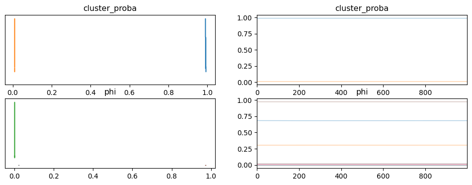
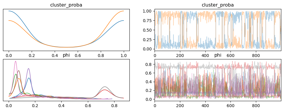
I think I am doing the log_prob calculation correctly as the two methods produce the same values for the same data, but when I try and fit the model using MCMC I don’t get anything like sensible results. The traces of cluster_proba jump back and forth between 0 and 1 during sampling when the clusters are about equally probable. This works with minor modifications (priors from a Beta distribution rather than a Dirichlet distribution for example) when using the builtin Bernoulli distribution that assumes independent variables, and also with a custom distribution that implements the independent Bernoulli distribution.

Does anyone have any ideas about what’s going wrong?

Many thanks!

check if the gradients of log_prob look reasonable?

How would I do that? Would something like jax.grad be the thing to use for this?

yes

Hi @martinjankowiak ,

Thanks for your help so far. I think the gradients are okay. I’ve done a bit more work and set up a google colab to demonstrate the problem here: Google Colab

I can run the model with one cluster, and it reproduces the correct parameters from the simulated data, but when I run the model with more than one cluster it puts all samples in one cluster and incorrectly estimates the coefficients. I assume the issue is that I’ve have defined the distribution incorrectly. I would be very grateful if you could take a look and give me some pointers.

Thanks :slight_smile:

Hi @martinjankowiak @fehiepsi . Sorry to be a pain, but I’d really appreciate it if you could have a look at this. I’m sure the solution will be something relatively simple but I don’t know where to look in the documentation to get any guidance on this.

Thanks

sorry but i have no idea what kind of distribution you’re aiming for and don’t have time to read up on it and code like

[jnp.array([v[j] for v, j in zip(zip(value.T, (1-value).T), i)]).prod(axis=0) 
                 for i in itertools.product(*[[0,1] for _ in range(value.shape[-1])])]

isn’t exactly transparent.

  • does your log_prob return the correct shapes? e.g. compare to the analogous log_prob for vanilla bernoulli
  • is prod going to be numerically stable? why not use log prod = sum log?

Thanks for your help. Here is the latest version linked above in the google colab ( Google Colab ).

class MultivariateBernoulli2D(dist.Distribution):
    # Note, this implementation is specifically
    # for two correlated Bernoulli variables
    support = dist.constraints.real_vector

    def __init__(self, phi_zero, phi_coef, phi_cross):
        super(MultivariateBernoulli2D, self).__init__(
            batch_shape=phi_coef.shape[:-1],
            event_shape=phi_coef.shape[-1:]
        )

        self.phi_zero = phi_zero
        self.phi_coef = phi_coef
        self.phi_cross = phi_cross

    def sample(self, key, sample_shape=()):
        raise NotImplementedError


    def log_prob(self, value):

        zeroth_term = self.phi_zero
        first_term = (value * self.phi_coef).sum(axis=-1)
        second_term = jnp.prod(value, axis=-1, keepdims=False) * self.phi_cross
        return zeroth_term + first_term + second_term

value above can either be zero or one, so prod(value) will be one when both values are one and zero otherwise. I don’t think there are any problems with numerical instability but let me know if I’ve got that wrong.

Here is the model.

@config_enumerate
def discrete_mixture_model(
    K,
    N,
    D_discrete,
    X_discrete=None,
):

    cluster_proba = numpyro.sample('cluster_proba', dist.Dirichlet(1.0 * jnp.ones(K)))

    # There are some places in the code to account for differences in tensor
    # shapes when the number of clusters is 1. Flagged here and in comments
    # below
    if K > 1:
        with numpyro.plate("discrete_cluster", K):
            phi = numpyro.sample('phi', dist.Dirichlet(1.0 * jnp.ones(2 ** D_discrete)))
    else:
        phi = numpyro.sample('phi', dist.Dirichlet(1.0 * jnp.ones(2 ** D_discrete)))

    # This is specific to the case of two correlated Bernoulli variables.
    phi_zero = jnp.log(phi[..., 0])
    phi_coef = jnp.array([jnp.log(phi[..., 1] / phi[..., 0]), jnp.log(phi[..., 2] / phi[..., 0])])
    phi_cross = jnp.log(phi[..., 0] * phi[..., 3] / (phi[..., 1] * phi[..., 2]))

    # K = 1
    if len(phi_zero.shape) == 0:
        phi_zero = jnp.array([phi_zero])
        phi_coef = phi_coef.reshape(1, -1)
        phi_cross = jnp.array([phi_cross])

    with numpyro.plate('data', N):

        assignment = numpyro.sample('assignment', dist.CategoricalProbs(cluster_proba))

        # K = 1
        if K == 1:
            target = MultivariateBernoulli2D(phi_zero, phi_coef, phi_cross)
        else:
            target = MultivariateBernoulli2D(phi_zero[assignment], phi_coef[assignment, :], phi_cross[assignment])

        numpyro.sample(
            'obs',
            target,
            obs=X_discrete,
        )

Here is the trace plot for the two cluster case

As you can see, all samples get erroneously dumped into one cluster.

For multivariate 2D, you can sum of probs over all possible values to check whether the implementation is correct or not. If the posterior is multimodal, then you need other mcmc algorithms.

Thanks. I’ve been working on this and I’m pretty sure the problem is in the log_prob method, specifically with the shape of each of the terms. Is there any documentation anywhere with details on how to create custom distributions for use in numpyro models? I guess the enumeration over the discrete latent variable is adding some complexity, but I’m really struggling to understand how things are working differently when the distribution is called from the model.

Thanks!

You can check how the shapes work at Tensor shapes in Pyro — Pyro Tutorials 1.9.0 documentation

d: batch_shape + event_shape
value: sample_batch_shape + event_shape
d.log_prob(value): broadcast_shapes(batch_shape, sample_batch_shape)

If you think this is the issue of log_prob, you can check:

  • whether sum of probs over all possible values is 1: e.g. you can try exp(d.log_prob(array([1, 0]))) + exp(d.log_prob(array([1, 1]))) + ...
  • whether the shapes satisfy the batch semantics above

The second one can be checked using vmap, i.e. comparing:

d(batch_phi).log_prob(value)

with

jax.vmap(lambda phi: d(phi).log_prob(value))(batch_phi)

If this is batch issue, check out the Writing parallelizable code¶ section at Tensor shapes in Pyro — Pyro Tutorials 1.9.0 documentation

1 Like

Hi @fehiepsi . Thanks again for your help.

I’ve modified the distribution code so all the checks you suggested work (I think) i.e.

phi_m = np.random.dirichlet(np.ones(4))
x = jnp.array([[0,0], [1,0], [0,1], [1,1]]) # this is all possible states
d_m = MultivariateBernoulli2D(phi_m)
print("sum check", jnp.exp(d_m.log_prob(x)).sum(axis=-1))

prints 1.0, and all the shape parameters of the distribution match the independent variables Bernoulli distribution dist.Bernoulli(phi).to_event(1).

Also, the jax vmap check that you suggested returns the same shape: (50, 4)

phi_m = np.random.dirichlet(np.ones(4), size=50)
print(MultivariateBernoulli2D(phi_m).log_prob(x).shape)
print(jax.vmap(lambda phi: MultivariateBernoulli2D(phi).log_prob(x))(phi_m).shape)

Unfortunately this still doesn’t fix the problem. Here is the distribution and model code:

class MultivariateBernoulli2D(dist.Distribution):
    support = dist.constraints.real_vector

    def __init__(self, phi):
        super(MultivariateBernoulli2D, self).__init__(
            batch_shape=phi.shape[:-1],
            event_shape= (2,)
        ) 
        
        self.phi = phi
        
    def sample(self, key, sample_shape=()):
        raise NotImplementedError
        
        
    def log_prob(self, value):

        val_m = 1 - value

        first_term = jnp.prod(value, axis=-1, keepdims=False) * jnp.log(self.phi[..., [0]])
        second_term = jnp.prod(jnp.concatenate([value[:, [0]], val_m[:, [1]]], axis=-1), axis=-1, keepdims=False) * jnp.log(self.phi[..., [1]])
        third_term = jnp.prod(jnp.concatenate([val_m[:, [0]], value[:, [1]]], axis=-1), axis=-1, keepdims=False) * jnp.log(self.phi[..., [2]])
        last_term = jnp.prod(val_m, axis=-1, keepdims=False) * jnp.log(self.phi[..., [3]])
        
        out = first_term + second_term + third_term + last_term
        
        return out.squeeze()


@config_enumerate
def discrete_mixture_model(
    K, 
    N, 
    D_discrete, 
    X_discrete=None,
):
    
    cluster_proba = numpyro.sample('cluster_proba', dist.Dirichlet(1.0 * jnp.ones(K))) 
    
    if K > 1:
        with numpyro.plate("discrete_cluster", K):
            phi = numpyro.sample('phi', dist.Dirichlet(2.0 * jnp.ones(2 ** D_discrete))) 
    else:
        phi = numpyro.sample('phi', dist.Dirichlet(2.0 * jnp.ones(2 ** D_discrete)))
    
    with numpyro.plate('data', N):
        
        assignment = numpyro.sample('assignment', dist.CategoricalProbs(cluster_proba)) 
        
        if K == 1:
            target = MultivariateBernoulli2D(phi) 
        else:
            target = MultivariateBernoulli2D(phi[assignment]) 
        
        
        out = numpyro.sample(
            'obs', 
            target,
            obs=X_discrete,
        )

Trace plot when fitting to data with 2 clusters:

Any ideas? Full code in the google colab: Google Colab

Could you compare vmap results, rather than just shapes? Then gradually add more dimensions. This will confirm that your log_prob is correct (in the sense of representing the log density of a distribution). Inference is another story (you might need to deal with label switching issues - i’m not sure).

The vmap method produces the same results as calling the log_prob directly, so I think that is working correctly. Do you know why there would be label switching problems with this but not with the built in Bernoulli distribution dist.Bernoulli(phi).to_event(1)?

Given cluster_proba and assignment, new_cluster_proba = 1 - cluster_proba and new_phi = 1 - phi (or its permutation), I feel like they will give you the same density. (I’m not sure what is the phi[..., 3] in your code, what do you mean by “such issue does not happen with the built in dist.Bernoulli(phi).to_event(1)”).

If I modify the model to use the distribution we discussed before in this thread: Mixture model with discrete data in Numpyro - #8 by jim (assuming independent Bernoullis) then I don’t get the label switching behaviour and all the model parameters are estimated pretty well. The change to this custom distribution does take a bit of modification to the model, as the parameters of the independent case are simple probabilities that I’ve used Beta priors and sampling for them, but the case here has a constraint that the parameters are a simplex so I need to use something like a Dirichlet prior instead.

Even without the label switching here, the model looks like it would still be dumping all observations in the same cluster, which is not what I want.

Thanks.

Do you think the posterior is easy to sample from (e.g. single modal)? If not, you might need Example: Neural Transport — NumPyro documentation or something else.

I’m pretty sure the posterior should be well behaved, ie single modal.