(Thanks to the developers for their hard work, I’m very happily considering converting Stan code to numpyro for a few projects!)
I’m interested in reproducing the results in Yao, Vehtari, Simpson & Gelman, “Yes, but Did It Work?: Evaluating Variational Inference” [ICML 2018] and have a short colab here that shows what’s going on (feel free to add comments inline): Google Colab
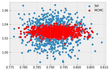
As their first example, Yao et al propose a linear regression model. I would think that since the mean-field assumption is actually satisfied, SVI would work quite well. The posterior means are perfectly recovered, but comparing MCMC to SVI shows that the variances seem to be systematically off. Anyone have ideas? Thanks!
Even if the mean field assumption is true for the true posterior, the true posterior may not be in the approximate posterior family Q. For example, Q could be mean-field Gaussian, and P could be mean-field laplace/student-t/etc, or P could be skewed.
In this case, the authors of the paper suggest that P is skewed to the right. You can think of mean field VI wanting to really avoid areas of low density, so the mean (not just the variance) getting pushing to the right, causing bias.
Other examples include when the ‘true posterior’ is a mean-field Laplace/student-t distribution (e.g., something with heavy tails). If the family of approximate posteriors if Gaussian (as is commonly the case), I would expect the approximate posterior q to underestimate the variance of the parameters - we can never find a q with KL(q||p)=0, and variational inference solutions always tend to be ‘more compact’ than the true posterior due to KL(q||p) integrating over q and having large penalty if p is small and q is large.
You could also imagine fitting a ‘mean-field’ true posterior that is a mixture of Gaussians for each component. Then mean field VI would probably ‘select’ a mode for each variable depending on the initialisation, therefore underestimating the posterior variance.
If you wanted to recover the mean and variance correctly, and the mean-field assumption is satisfied, you’d probably be better off using EP (expectation propagation, which moment matches for exponential families), but I don’t know how this works with probabilistic programming languages.
2 Likes
Thanks Mrinank. To clarify, the posterior here really is close to Gaussian! And SVI is overstating uncertainty, rather than understating it, which I don’t think is typical.
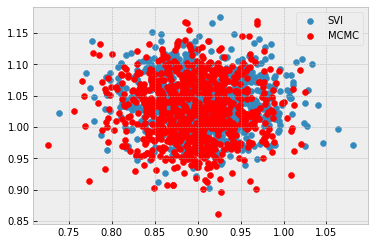
To make the posterior more Gaussian, I’ve simplified the example, fixing the noise parameter sigma. Somehow the performance is even worse for sigma = 0.5, but sigma = 5.0 seems to work.
Other suggestions to try? Tweaks to the optimization/initialization?
sigma = 0.5:
sigma = 5.0:
Here’s the notebook: Google Colab
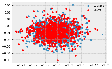
For sanity checking, I’ve tried Laplace and it works fine on both examples, fixed sigma and prior on sigma.
I’d suggest initialising the variance of MFVI to be quite tight (maybe 1e-5 or so) to see if it behaves similarly. With a fixed value of sigma, the behaviour is confusing and could be optimisation/initialisation related.
It might be worth seeing if full-batch VI (i.e., very large batch size, or reduce number of examples) has qualitatively similar performance too.
When sigma is learnt, it could be instead that VI is ‘underestimating uncertainty’ in sigma, which doesn’t mean that the predictive posterior will necessarily be tighter for VI. In other words, I think we need to reason in parameter space rather than the predictive posterior.
A larger batch size seems to fix it! Notebook here. Question for anyone who knows—is this the right way to make stochastic gradient descent regular gradient descent? Or is this sampling with replacement? n is the sample size:
svi = SVI(model, guide, optimizer, loss=Trace_ELBO(num_particles=n))