Beginner question on SVI: how to find parameters of a normal distribution

[adk]

I have a conceptual problem getting Pyro to learn the parameters of a distribution using SVI. For some reason, SVI is not correctly learning the sigma/scale parameter of a normal distribution. Here is the problem setup:

%matplotlib notebook
import numpy as np
import matplotlib.pyplot as plt
from pyro.optim import Adam
from pyro.infer import SVI, Trace_ELBO
import pyro
import torch
from tqdm.notebook import tqdm

mu_prior = 42.0
sigma_prior = 1.0

def model(obs):
    with pyro.plate("samples",len(obs)):
        s = pyro.sample("test", dist.Normal(mu_prior,sigma_prior), obs = obs)
   
def guide(obs):
    mu_param = pyro.param('mu_param',torch.tensor(mu_prior))
    sigma_param = pyro.param('sigma_param',torch.tensor(sigma_prior))
    with pyro.plate("samples",len(obs)):
        s = pyro.sample("test",dist.Normal(mu_param,sigma_param))
    
adam_params = {"lr": 0.005, "betas": (0.95, 0.999)}
optimizer = Adam(adam_params)

svi = SVI(model, guide, optimizer, loss=Trace_ELBO(num_particles=100))

obs = torch.tensor(np.random.normal(loc=mu_prior,scale=sigma_prior,size=1000))

I would like SVI to learn mu and sigma, the parameters of the distribution. To keep things simple, I am sampling from the prior distribution to make sure that the posterior is the same as the prior. To learn the parameters, I run the following:

fig = plt.figure(figsize=(8,16))
ax1 = fig.add_subplot(311)
ax2 = fig.add_subplot(312)
ax3 = fig.add_subplot(313)

axes = ax1,ax2,ax3
plt.ion()

pyro.clear_param_store()
n_steps=20000
loss = []
mu = []
sigma = []
for step in tqdm(range(n_steps)):
    l = svi.step(obs)
    loss.append(l)
    mu.append(pyro.param('mu_param').item())
    sigma.append(pyro.param('sigma_param').item())
    
    for ax in axes:
        ax.clear()
    ax1.plot(loss,label="loss")
    ax1.title.set_text("training loss")
    ax2.plot(mu,label="mu")
    ax2.title.set_text("mu")
    ax3.plot(sigma,label="sigma")
    ax3.title.set_text("sigma")
    fig.canvas.draw()

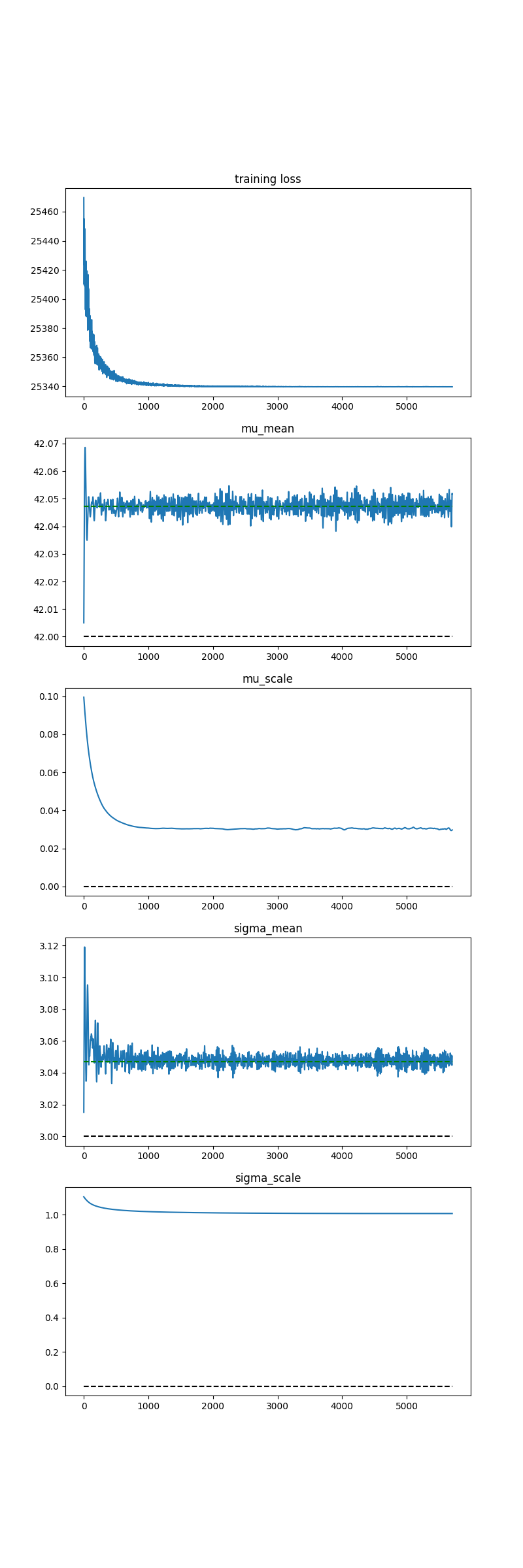
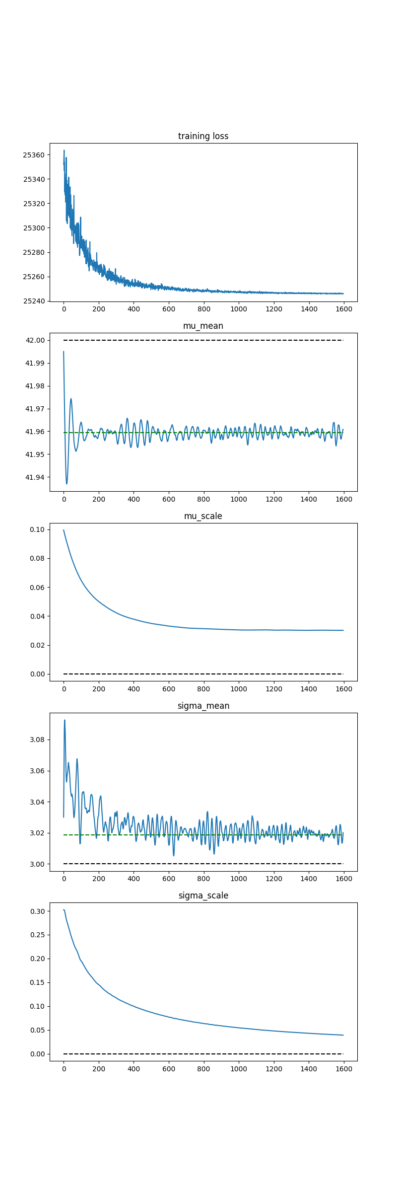
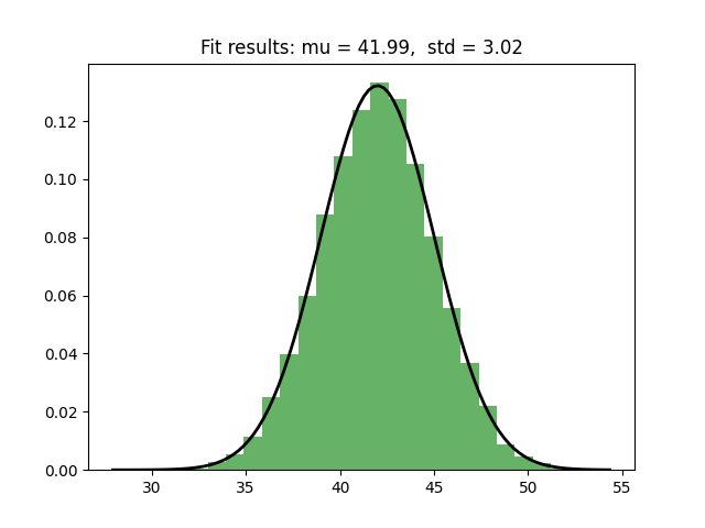
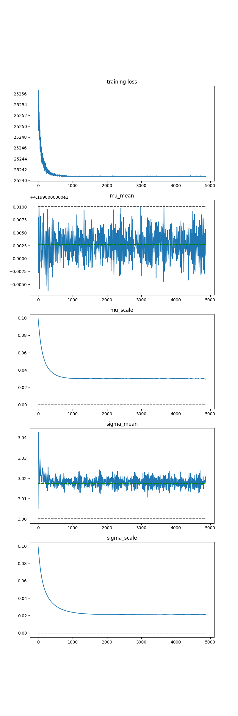
The output is:

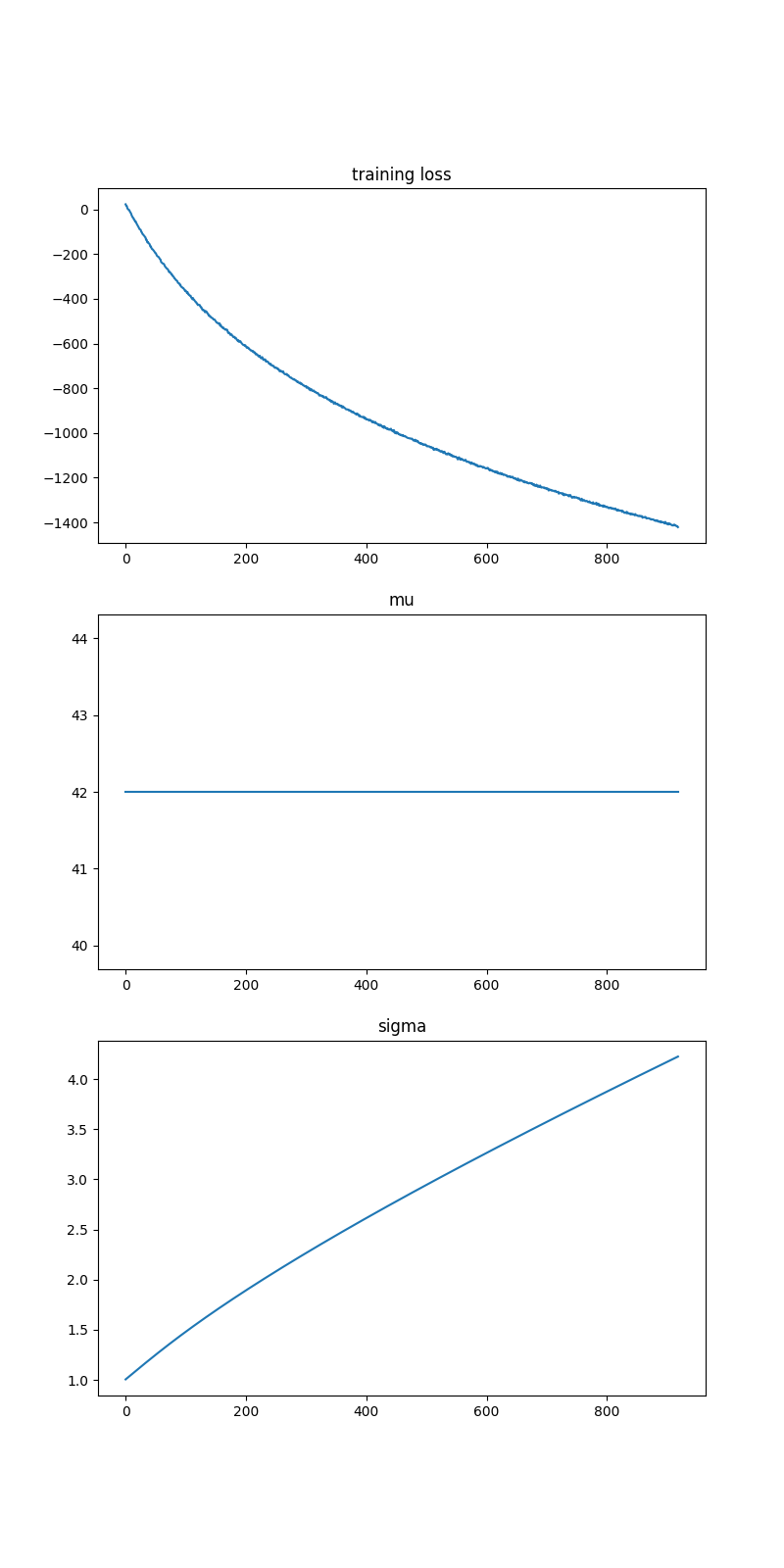
The mean (mu) parameter is correct, but the scale parameter just continues to grow as I run SVI for more iterations. Clearly I’m missing something fundamental, but I’m at a loss. Can anyone help?

[fritzo]

1. In Bayesian inference your model will need latent variables. Currently it has no latent variables.
2. The guide should merely sample the latent variables, not the likelihood.
3. Careful with scale parameters, they should be constrained positive.

from pyro.distributions import constraints

def model(obs):
    mu = pyro.sample("mu", dist.Normal(mu_prior, 1.0))
    sigma = pyro.sample("sigma", dist.LogNormal(math.log(sigma_prior), 1.0))
    with pyro.plate("samples",len(obs)):
        pyro.sample("test", dist.Normal(mu, sigma),
                    obs=obs)

def guide(obs):
    mu_mean = pyro.param('mu_mean', torch.tensor(mu_prior))
    mu_scale = pyro.param('mu_scale', torch.tensor(0.1),
                          constraint=constraints.positive)
    sigma_log_mean = pyro.param('sigma_log_mean', torch.tensor(math.log(sigma_prior))))
    sigma_log_scale = pyro.param('sigma_log_scale', torch.tensor(0.1),
                                 constraint=constraints.positive)
    pyro.sample("mu", dist.Normal(mu_mean, mu_scale)
    pyro.sample("sigma", dist.LogNormal(sigma_log_mean, sigma_log_scale))

[adk]

Thank you very much for the help! One clarification: I think you may have meant

sigma = pyro.sample("sigma", dist.LogNormal(math.log(sigma_prior), 1.0))

so that the sample site has the same name in model and guide. Is that correct? and

pyro.sample("mu", dist.Normal(mu_mean, mu_scale))

(mu is sampled from Normal rather than LogNormal)

Thanks again!

[fritzo]

Good catches! I’ve added your fixes to my answer so as to avoid confusing future readers

[adk]

I wanted to follow up with some new questions. when I run SVI on the model and guide in @fritzo 's code above, I notice that that the mu_mean and sigma_mean parameters do exactly what I’d expect, but I’m not sure how to interpret the mu_scale and sigma_scale parameters. Specifically, I have generated data to fit in the following way:

mu_prior = 42.0
sigma_prior = 3.0
obs = torch.tensor(np.random.normal(loc=mu_prior,scale=sigma_prior,size=10000))

that is, the data are generated from a normal distribution with a fixed mu and sigma. I fit a normal distribution to the resulting 10,000 points as a sanity check:

from scipy.stats import norm

obs_arr = np.array(obs)

mu_fit, sigma_fit = norm.fit(obs_arr)

# Plot the histogram.
plt.hist(obs_arr, bins=25, density=True, alpha=0.6, color='g')

# Plot the PDF.
xmin, xmax = plt.xlim()
x = np.linspace(xmin, xmax, 100)
p = norm.pdf(x, mu_fit, sigma_fit)
plt.plot(x, p, 'k', linewidth=2)
title = "Fit results: mu = %.2f,  std = %.2f" % (mu_fit, sigma_fit)
plt.title(title)

plt.show()

The fit mu parameter is 42.05, and the fit sigma parameter is 3.05. When I run SVI I see the following parameter values over time:

The green dashed lines are the values found by scipy’s norm.fit(), and the black dashed lines are the true parameters of the data distribution. I notice that the mu_mean and sigma_mean parameters found by Pyro are, on average, very close to those found by norm.fit(). The question is, what is the meaning of the mu_scale and sigma_scale parameters? Are they junk, because mu and sigma are actually not sampled from normal distributions, or do they have some interpretable meaning as the “confidence” in the values of mu_mean and sigma_mean that SVI found?

Thanks again!

[fritzo]

@adk

do they have some interpretable meaning as the “confidence” in the values of mu_mean and sigma_mean that SVI found?

Yes exactly, these parametrize the variational posterior uncertainty of the two parameters you’ve estimated. As an educational exercise, you might try training the model on each of [1, 10, 100, 1000, 10000] datapoints, i.e. subsetting your data, and plot how all the learned parameters change as your data grows. You should expect the mu_mean and sigma_mean parameters to noisily converge to the true values, and the mu_scale and sigma_scale to decrease according to 1/sqrt(len(data)); this illustrates the Bernstein-von Mises Theorem.

[adk]

I don’t understand the nuances of the bernstein-von Mises Thm but it is intuitive that uncertainty in parameter estimates should decrease as the number of observed data increases. What I’m having trouble with is that the uncertainty measure for the sigma variable (sigma_scale) that SVI finds seems high in this case. By comparison, mu_scale seems to better reflect reality in this example: the actual mu value is 42, the mu_mean parameter found is approximately 42.046 and the mu_scale parameter is 0.03, putting the parameter estimate about one standard dev from the true value. The true sigma value was 3.0, the sigma_mean parameter ended up quite close to the true value at about 3.045, but the sigma scale parameter stayed quite large, at 1.0. Can you give some insight into this disparity?

Thanks!

edit: the prior on mu_scale and sigma_scale, used in the sample() statements in the model function were both 1.0 as in your first reply.

[fritzo]

I don’t know why sigma_scale is so high. It would help to know what sigma_scale is and what it was initialized to; it appears the plots were generated with a different model and guide from the one I pasted above.

[adk]

the full code for this example is:

#imports
%matplotlib notebook
import numpy as np
import math
import matplotlib.pyplot as plt
from pyro.optim import Adam
from pyro.infer import SVI, Trace_ELBO
import pyro
import torch
from tqdm.notebook import tqdm
import pyro.distributions as dist
from pyro.distributions import constraints

#model and guide definitions
mu_prior = 42.0
sigma_prior = 3.0

def model(obs):
    mu = pyro.sample("mu", dist.Normal(mu_prior, 1.0))
    sigma = pyro.sample("sigma", dist.LogNormal(math.log(sigma_prior), 1.0))
    with pyro.plate("samples",len(obs)):
        pyro.sample("test", dist.Normal(mu, sigma),
                    obs=obs)

def guide(obs):
    mu_mean = pyro.param('mu_mean', torch.tensor(mu_prior))
    mu_scale = pyro.param('mu_scale', torch.tensor(0.1),
                          constraint=constraints.positive)
    sigma_log_mean = pyro.param('sigma_log_mean', torch.tensor(math.log(sigma_prior)))
    sigma_log_scale = pyro.param('sigma_log_scale', torch.tensor(0.1),
                                 constraint=constraints.positive)
    pyro.sample("mu", dist.Normal(mu_mean, mu_scale))
    pyro.sample("sigma", dist.LogNormal(sigma_log_mean, sigma_log_scale))

#optimizer and SVI setup
adam_params = {"lr": 0.005, "betas": (0.95, 0.999)}
optimizer = Adam(adam_params)
svi = SVI(model, guide, optimizer, loss=Trace_ELBO(num_particles=100))

#sample data generation:
obs = torch.tensor(np.random.normal(loc=mu_prior,scale=sigma_prior,size=10000))

#fitting a distribution with scipy.stats.norm:
from scipy.stats import norm

obs_arr = np.array(obs)

mu_fit, sigma_fit = norm.fit(obs_arr)

# Plot the histogram.
plt.hist(obs_arr, bins=25, density=True, alpha=0.6, color='g')

# Plot the PDF.
xmin, xmax = plt.xlim()
x = np.linspace(xmin, xmax, 100)
p = norm.pdf(x, mu_fit, sigma_fit)
plt.plot(x, p, 'k', linewidth=2)
title = "Fit results: mu = %.2f,  std = %.2f" % (mu_fit, sigma_fit)
plt.title(title)

plt.show()

#running inference & visualizing output:
fig = plt.figure(figsize=(8,24))
ax1 = fig.add_subplot(511)
ax2 = fig.add_subplot(512)
ax3 = fig.add_subplot(513)
ax4 = fig.add_subplot(514)
ax5 = fig.add_subplot(515)

axes = ax1,ax2,ax3,ax4,ax5
plt.ion()

pyro.clear_param_store()
n_steps=20000
loss = []
mu_scale = []
mu_mean = []
sigma_log_mean = []
sigma_log_scale = []
for step in tqdm(range(n_steps)):
    l = svi.step(obs)
    loss.append(l)
    mu_mean.append(pyro.param('mu_mean').item())
    mu_scale.append(pyro.param('mu_scale').item())
    sigma_log_mean.append(pyro.param('sigma_log_mean').item())
    sigma_log_scale.append(pyro.param('sigma_log_scale').item())
    
    for ax in axes:
        ax.clear()
    ax1.plot(loss)
    ax1.title.set_text("training loss")
    ax2.plot(mu_mean)
    ax2.title.set_text("mu_mean")
    ax2.hlines(mu_prior,0,len(mu_mean),linestyles='dashed',color='black')
    ax2.hlines(mu_fit,0,len(mu_mean),linestyles='dashed',color='green')
    ax3.plot(mu_scale)
    ax3.title.set_text("mu_scale")
    ax3.hlines(0,0,len(mu_scale),linestyles='dashed',color='black')
    ax4.plot(np.exp(sigma_log_mean))
    ax4.title.set_text("sigma_mean")
    ax4.hlines(sigma_prior,0,len(sigma_log_mean),linestyles='dashed',color='black')
    ax4.hlines(sigma_fit,0,len(sigma_log_mean),linestyles='dashed',color='green')
    ax5.plot(np.exp(sigma_log_scale))
    ax5.title.set_text("sigma_scale")
    ax5.hlines(0,0,len(sigma_log_scale),linestyles='dashed',color='black')
    fig.canvas.draw()

edit: this is a naive guess, but could the larger-than-expected sigma_scale have to do with sampling from a log-normal distribution rather than from a normal distribution with positive constraints enforced on sigma_mean and sigma_scale?

[fritzo]

Looks like this is just a plotting error Where you write

@adk

ax5.plot(np.exp(sigma_log_scale))

I believe this should instead be

ax5.plot(sigma_log_scale)

since sigma_log_scale is the positive scale parameter of log(sigma). If you want to convert this to a proper mean and standard deviation, you could use the LogNormal properties

d = dist.LogNormal(sigma_log_mean, sigma_log_scale)
ax4.plot(d.mean)
ax5.plot(d.variance.sqrt())

[adk]

Wasn’t just a plotting issue, it was genuine confusion. It seems to me that both sigma_log_mean and sigma_log_scale should be in logarithmic units, and I’m still not sure why sigma_log_scale would be the appropriate variable to plot for sigma_scale. However, when I replace my plotting code with a slightly modified version of your suggestion above:

    dists = [dist.LogNormal(lm, ls) for lm,ls in zip(sigma_log_mean,sigma_log_scale)]
    sigma_mean = [d.mean for d in dists]
    sigma_scale = [d.variance.sqrt() for d in dists]
    ax4.plot(sigma_mean)
    ...
    ax5.plot(sigma_scale)

then I believe it is doing the right conversion, and the values for sigma_scale that the optimizer finds seem more reasonable:

edit: so, clearly it was a mistake for me to plot exp(sigma_log_scale), and I believe the code above corrects it even though I don’t completely understand the conversion it is doing, but I still don’t understand why sigma_log_scale would represent the standard dev of the sigma parameter.

[fritzo]

sigma_log_scale represents the standard deviation of the log of the sigma parameter because that’s just how LogNormal is parametrized. But note the standard-deviation-of-the-log is different from the log-of-the-standard-deviation, so that exp(stddev(log(sigma))) isn’t the same as stddev(exp(log(sigma))) = stddev(sigma). I think this was the source of the plotting error.

Anyway, glad to see some more plausible plots

[adk]

@fritzo , I can’t thank you enough for the follow up, this is very helpful. On the subject of LogNormal, it’s my understanding that you used it here just because it happens to only output positive values, not because there is some deeper reason that a scale parameter for a normal distribution should be sampled from LogNormal. If I’m right in thinking that, we could also ensure positivity in other ways. I tried the following redefinition of model and guide to eliminate the use of LogNormal:

#imports as before
#model and guide definition:
mu_prior = 42.0
sigma_prior = 3.0

def model(obs):
    mu = pyro.sample("mu", dist.Normal(mu_prior, 1.0))
    sigma = pyro.sample("sigma", dist.Normal(sigma_prior, 1.0))
    if sigma < 0: #is this a viable way of ensuring sigma is positive, without using LogNormal?
        sigma = sigma * -1
    with pyro.plate("samples",len(obs)):
        pyro.sample("test", dist.Normal(mu, sigma),
                    obs=obs)

def guide(obs):
    mu_mean = pyro.param('mu_mean', torch.tensor(mu_prior))
    mu_scale = pyro.param('mu_scale', torch.tensor(0.1),
                          constraint=constraints.positive)
    sigma_mean = pyro.param('sigma_mean', torch.tensor(sigma_prior))
    #constraint=constraints.positive)#pos constraint no longer needed because of conditional sign flip in model
    sigma_scale = pyro.param('sigma_scale', torch.tensor(0.1),
                                 constraint=constraints.positive)
    pyro.sample("mu", dist.Normal(mu_mean, mu_scale))
    pyro.sample("sigma", dist.Normal(sigma_mean, sigma_scale))

In other words, instead of sampling sigma from LogNormal, sample it from abs(Normal(.))

#svi and optimizer
adam_params = {"lr": 0.005, "betas": (0.95, 0.999)}
optimizer = Adam(adam_params)
svi = SVI(model, guide, optimizer, loss=Trace_ELBO(num_particles=100))
#data samples
obs = torch.tensor(np.random.normal(loc=mu_prior,scale=sigma_prior,size=10000))

our data look like:

fig = plt.figure(figsize=(8,24))
ax1 = fig.add_subplot(511)
ax2 = fig.add_subplot(512)
ax3 = fig.add_subplot(513)
ax4 = fig.add_subplot(514)
ax5 = fig.add_subplot(515)

axes = ax1,ax2,ax3,ax4,ax5
plt.ion()

pyro.clear_param_store()
n_steps=20000
loss = []
mu_scale = []
mu_mean = []
sigma_mean = []
sigma_scale = []
for step in tqdm(range(n_steps)):
    l = svi.step(obs)
    loss.append(l)
    mu_mean.append(pyro.param('mu_mean').item())
    mu_scale.append(pyro.param('mu_scale').item())
    sigma_mean.append(pyro.param('sigma_mean').item())
    sigma_scale.append(pyro.param('sigma_scale').item())
    
    
    for ax in axes:
        ax.clear()
    ax1.plot(loss)
    ax1.title.set_text("training loss")
    ax2.plot(mu_mean)
    ax2.title.set_text("mu_mean")
    ax2.hlines(mu_prior,0,len(mu_mean),linestyles='dashed',color='black')
    ax2.hlines(mu_fit,0,len(mu_mean),linestyles='dashed',color='green')
    ax3.plot(mu_scale)
    ax3.title.set_text("mu_scale")
    ax3.hlines(0,0,len(mu_scale),linestyles='dashed',color='black')
    ax4.plot(sigma_mean)
    ax4.title.set_text("sigma_mean")
    ax4.hlines(sigma_prior,0,len(sigma_mean),linestyles='dashed',color='black')
    ax4.hlines(sigma_fit,0,len(sigma_mean),linestyles='dashed',color='green')
    ax5.plot(sigma_scale)
    ax5.title.set_text("sigma_scale")
    ax5.hlines(0,0,len(sigma_scale),linestyles='dashed',color='black')
    fig.canvas.draw()

Running this code produces:

This also seems to produce sane values for mu_scale and sigma_scale in addition to learning the mean parameters correctly. Is this a good approach too or is it conceptually lacking?

[fritzo]

That’s also a valid model, and it is equivalent to using a HalfNormal or FoldedDistribution(Normal(…)) variational posterior for sigma. I believe the true posterior over sigma (conditioned on mu) is an inverse Gamma distribution, but the true joint posterior is more complex. I usually use Normal for real-valued variational posteriors and LogNormal for positive-valued posteriors. When I expect posterior correlation I use AutoLowRankMultivariateNormal guides.

[adk]

Just to clarify what you mean by expecting posterior correlation: when you don’t know how the variables are correlated (other than expecting covariance to be be low rank) you use AutoLowRankMultivariateNormal, but if you know the dependence structure of your variables (that is, you understand the program that determines how the latent variables are correlated but not the distributions over the variables themselves) would you then construct the guide to sample the latent variables using this known program? (thus replicating the part of the program that samples the latent variables, between model and guide, with the key difference that the guide sampling process has variable parameters whereas the distribution parameters in the model are fixed)

[fritzo]

You could in principle write a custom guide that encapsulates a know dependency structure, but I only use autoguides and automatic structured guides. I find there’s usually more to be gained in fast model iteration than in tediously improving the variational distribution for a single particular model.

[adk]

OK, thanks. so If I understand correctly, you mean that it is better to invest effort in designing the model, using a sufficiently general (perhaps too general) guide, and let SVI discover the covariance matrix of the guide distribution. Even when we know that certain elements of the covariance matrix will be 0, because of our prior knowledge about the dependence structure of the latent variables. If this is what you mean, then I assume optimizing the guide would only offer a small savings in computational cost, at the risk of introducing errors through programming mistakes in the guide distribution.

On a related note, I wanted to verify my understanding of the meaning of the num_particles argument to the loss used in SVI. Is it the case that this is just the number of samples drawn from the guide at each step? And these samples are used to approximate the evidence lower bound, which we seek to maximize via optimization in the parameter space (thus decreasing the KL divergence between the true posterior over the latents and the guide).

[fritzo]

@adk

it is better to invest effort in designing the model

Yes, I find it’s best to optimize your workflow for fast model iteration, so you can make as many design cycles as possible through Box’s loop. I used to think hard about guides, but now I think much harder about models. Usually I can get good enough performance with AutoNormal, AutoLowRankMultivariateNormal, and AutoReparam, and crucially those don’t need to be changed each time I modify the model. That makes it easier to modify the model and easier to automatically search over tens or hundreds of model structures.

@adk

[num_particles] is just the number of samples drawn from the guide at each step

Correct. This is useful in small models, where vectorizing over 10-100 particles can often speed up inference by reducing the gradient noise and thus the number of learning steps needed for convergence.

[adk]

Thanks. From the docs, “…Autoguide packs the latent variables into a single tensor, in this case, one entry per variable sampled in our model…” Are the latents in the order that they first appear (first sample() statement in the model?) Is there a more explicit way to get the correspondences between the named latent variables and the indices into the .scale and .loc parameters generated by the autoguide?

[fritzo]

@adk

Is there a more explicit way to get the correspondences between the named latent variables and the indices into the .scale and .loc

The easiest way is to use AutoContinuous._unpack_latent() , and it’s not that easy. Indexing in a general way is pretty hard.