The jupyter notebook containing all the code can be seen here
Problem summary:
-
SVI for bayesian linear regression give very unreasonable posterior weights and noise level
-
The Trace_ELBO for the conjugate posterior seems to be larger than the optimized Trace_ELBO
After having read the basic pyro tutorial, I want to implement Bayesian linear regression on a toy dataset to verify my understanding of basic pyro concepts.
The dataset is a 1D linear function with randomly generated weights and pre-knowen noise level:
import torch
import pyro
import pyro.optim
import matplotlib.pyplot as plt
from torch.distributions import constraints

# The true model, with randomly generated weights and fixed noise level
noise_level = 0.1
w = torch.randn(1)
b = torch.randn(1)
xs = torch.randn(2000)
ys = w * xs + b
ys += torch.distributions.Normal(0,noise_level).sample(ys.shape)
plt.plot(xs.numpy(), ys.numpy(),'+')
print('w is %g, b is %g, noise_level is %g' % (w,b,noise_level))
Conjugate priors(Gaussian for the weights and Gamma for the precision) are used to define the model and guide, so that I can compare results with the exact posterior:
# The prior
def model(x,y):
    prec = pyro.sample("precision", pyro.distributions.Gamma(5,5))
    wb   = pyro.sample("wb", pyro.distributions.MultivariateNormal(torch.zeros(2), torch.eye(2)))
    for i in pyro.plate("data_loop", len(x), subsample_size=256):
        pyro.sample("obs_{}".format(i), pyro.distributions.Normal(wb[0] * x[i] + wb[1], torch.sqrt(1/prec)))

# The variational distribution
def guide(x,y):
    mu_wb = pyro.param("mu_wb", torch.zeros(2))
    L_wb    = pyro.param("L_wb", torch.eye(2), constraint = constraints.lower_cholesky)


    prec_a = pyro.param("prec_a", torch.tensor(5.), constraint = constraints.positive)
    prec_b = pyro.param("prec_b", torch.tensor(5.), constraint = constraints.positive)

    wb   = pyro.sample("wb", pyro.distributions.MultivariateNormal(mu_wb, L_wb.mm(L_wb.t())))
    prec = pyro.sample("precision", pyro.distributions.Gamma(prec_a, prec_b))
    return wb, prec

optimizer = pyro.optim.SGD({"lr": 1e-4, "momentum": 0.1})
pyro.clear_param_store()
svi = pyro.infer.SVI(model, guide, optimizer, loss=pyro.infer.Trace_ELBO())
rec_loss = []
for i in range(100):
    loss = svi.step(xs,ys)
    rec_loss.append(loss)
    print('Iter %d, loss = %g' % (i,loss))
After 100 SGD iterations, I drawn several samples from the posterior and have them plotted:
fig = plt.figure(figsize = (18,6))
plt.subplot(131)
plt.plot(rec_loss)

plt.subplot(132)
plt.plot(xs.numpy(),ys.numpy(),'+')
for i in range(10):
    wb, prec = guide(xs,ys)
    py = wb[0] * xs + wb[1]
    plt.plot(xs.numpy(), py.detach().numpy(), 'g', alpha = 0.1)


plt.subplot(133)
noise  = []
for i in range(1000):
    wb,prec = guide(xs,ys)
    noise.append(1/torch.sqrt(prec).item())
plt.hist(noise)
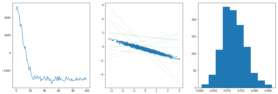
As can be seen, although considerable loss drop can be seen, the fitted model is very bad, the noise level seems to be highly underestimated, while the posterior weights just don’t make any sense.
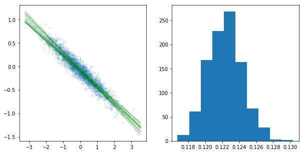
In the meantime, weights drawn from the analytical conjugate posterior distribution fit the data very well:
v0 = torch.eye(2)
n   = xs.shape[0]
x_aug = torch.ones(n,2)
x_aug[:,0] = xs

Vn = torch.inverse(torch.eye(2) + x_aug.t().mm(x_aug))
wn = Vn.mv(x_aug.t().mv(ys))
alpha_n = 5 + n / 2
beta_n   = 5 + 0.5 * (ys.dot(ys) - wn.dot(Vn.inverse().mv(wn)))

w_sampler = pyro.distributions.MultivariateNormal(wn,Vn)
prec_sampler = pyro.distributions.Gamma(alpha_n,beta_n)

plt.figure(figsize=(10,5))
plt.subplot(121)
plt.plot(xs.numpy(), ys.numpy(), '+', alpha = 0.2)
for i in range(10):
    wb = w_sampler.sample()
    py = wb[0]  * xs + wb[1]
    plt.plot(xs.numpy(), py.detach().numpy(), 'g', alpha = 0.3)

prec = torch.sqrt(1/prec_sampler.sample((1000,)))
plt.subplot(122)
plt.hist(prec.numpy())
The optimized ELBO is about -1500, and then I want to compare it with the ELBO of the analytical conjugate posterior with the below code:
def new_guide(x,y):
    wb   = pyro.sample("wb", pyro.distributions.MultivariateNormal(wn, Vn))
    prec = pyro.sample("precision", pyro.distributions.Gamma(alpha_n, beta_n))
    return wb, prec
new_svi = pyro.infer.SVI(model, new_guide, optimizer, pyro.infer.Trace_ELBO())
print(new_svi.step(xs,ys))
The result of the abolve code is about -1100, which seems to indicate a larger ELBO than the SGD-optimized value