I am trying to create a simple program representing the factor graph below:
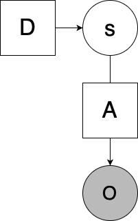
Where s = Cat(D) (so s is sampled from a vector D, which is a standard simplex; in the above graph it represents prior beliefs about the value of s), and o = As (where A is a matrix mapping latent values of s to observation space o). o and s will be one-hot vectors to represent discrete states and observations.
Below I have my attempt to create this in Pyro with a simple example, using two possible values of o and s (which means A is 2x2. Of course, in this simple model s could be solved analytically, but I wanted to experiment to see if I could get it working in Pyro. My confusion is with regards to constructing the guide in this case. I have tried it with/without the simplex constraint, but adding the simplex constraint to the sd parameter doesn’t seem to work (the final value for sd yielding [1,1].
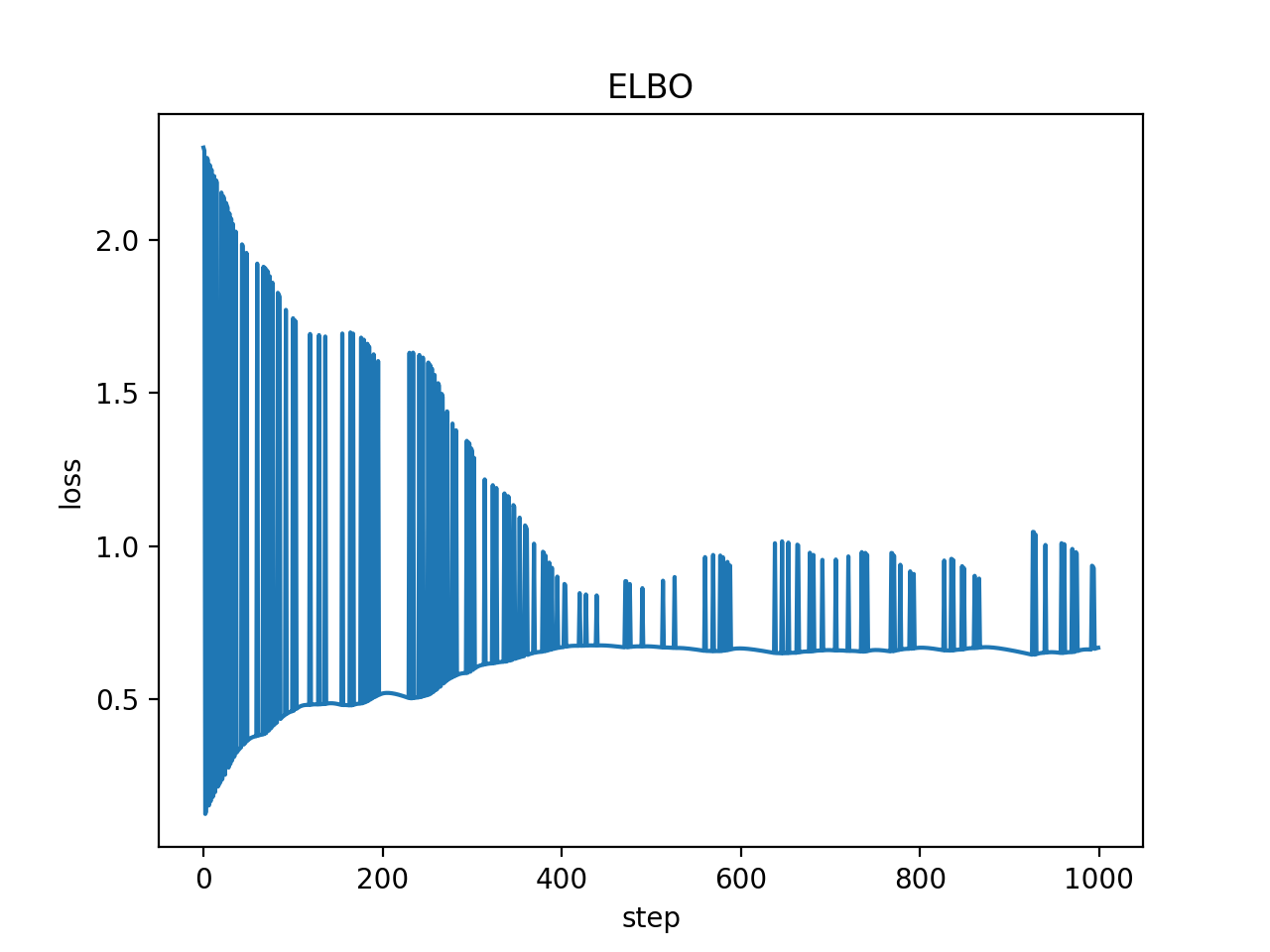
Even without the simplex constraint (using dist.constraints.positive in the below example), sd approaches the correct value (which, analytically, I believe should be [.96, .04] for the given values of D, A, and ob, reflecting the posterior beliefs in the value of s), but is still quite inconsistent across runs, and even the value it finishes on is not quite as close to what I would want. Furthermore, the plot of losses fluctuates quite a bit, which I believe is indicative of the underlying issue.
My hunch is that it has something to with my choice of distribution in my guide, but I’m not sure exactly what to use otherwise. Any help is appreciated!
import pyro
import torch
from torch import tensor

import pyro.distributions as dist
from pyro.optim import Adam
from pyro.infer import SVI, Trace_ELBO

import matplotlib.pyplot as plt
import numpy as np

from torch.nn import Softmax

A = tensor([
    [0.9, 0.1],
    [0.1, 0.9]
])

D = tensor([
    [0.5],
    [0.5]
])

Ns = D.shape[0]

def one_hot(num, sz):
    mat = torch.zeros([1, sz])
    mat[0][num] = 1.
    return mat.T

def model(o):
    s = pyro.sample("s",
        dist.Categorical(D.T)
    )

    s = one_hot(s, Ns)
    As = torch.matmul(A, s)

    pyro.sample("o",
        dist.Categorical( As.T ),
        obs = o
    )

def guide(o):
    sd = pyro.param("sd", tensor([
        [0.5],
        [0.5]
    ]), constraint = dist.constraints.positive)

    s = pyro.sample("s", dist.Categorical(sd.T))

adam = Adam({"lr": 0.1, "betas": (0.90, 0.999)})
svi = SVI(model, guide, adam, loss=Trace_ELBO())

param_vals = []
losses = []

ob = tensor([0])

for _ in range(1000):
    losses.append(svi.step(ob))
    param_vals.append({k: pyro.param(k) for k in ["sd"]})

plt.plot(losses)
plt.title("ELBO")
plt.xlabel("step")
plt.ylabel("loss")
plt.show()

fm = Softmax(dim=0)

print(fm(param_vals[-1]["sd"]))