Hi, I am hoping to get some help with a problem I am experiencing. I am facing an issue with marginalizing a latent discrete variable in numpyro. My latent variable depends on a high-order continuous variable, and when attempting to marginalize it, I encounter a large number of divergences due to the complex structure. I am wondering if I am making any errors in the process of marginalizing this latent discrete variable.
I have noticed that when I constrain the slope \lambda_{k} of the high-order continuous variable to the latent discrete variable to be 1, the model does not encounter divergences. However, when I allow the slope parameter to be freely estimated, I encounter a large number of divergences. Is there a need for additional reparameterization of the slope parameter?
Any help will be greatly appreciated.
The schematic diagram of the model is shown below:

The model code are as follows:
Data generate:
import numpy as np
import jax
from jax import nn, random, vmap
import jax.numpy as jnp
import numpyro
from numpyro import handlers
import numpyro.distributions as dist
from numpyro.infer import MCMC, NUTS, Predictive, DiscreteHMCGibbs, MixedHMC, HMC
from numpyro.infer.reparam import LocScaleReparam
from numpyro.ops.indexing import Vindex
from numpyro.handlers import reparam
import itertools
import arviz as az
numpyro.set_host_device_count(2)
import numpy as np
import itertools


I = 20 # number of item
K = 4 # number of attribute
N = 100 # number of respondent

# higher-order ability of repondent
theta = np.random.normal(0,1,(N,1))
# intercept: theta -> alpha
lam_0 = np.random.normal(0,2,(1,K))
# slope: theta-> alpha
lam_1 = np.random.lognormal(1,0.25,(1,K))
# attribute master prob
alpha_prob = nn.sigmoid(lam_0+lam_1*theta)
alpha = np.random.binomial(1,alpha_prob)

# slipping parameter of item
s = np.random.uniform(0.1,0.2, (1, I))
# guessing parameter of item
g = np.random.uniform(0.1,0.2, (1, I))

# all possible attribute profile 2^K
all_p = np.array(list(itertools.product(*[[0,1] for k in range(4)])))
all_p = all_p[np.argsort(all_p.sum(axis=-1))]

# Q matrix random generate
Q = np.concatenate([all_p[1:K+1], all_p[np.random.randint(1,len(all_p),I-K)]],axis=0)
# is respondent mastered all attribute required by item
xi = (alpha.reshape(N,1,K)>=Q.reshape(1,I,K)).prod(axis=-1)
# repondent correct prob
p = xi*(1-s-g)+g
Y = np.random.binomial(1,p)
Model construct
 #  if or not mastered all attribute required by item for category
cat_xi = jnp.asarray(all_p.reshape(2**K,1,K)>=Q.reshape(1,I,K)).prod(axis=-1)
 def HO_DINA(all_p):
# with numpyro.handlers.seed(rng_seed=0):
        respondent_plate = numpyro.plate("respondent", N, dim=-2)
        item_plate = numpyro.plate("item", I, dim=-1)
        att_plate = numpyro.plate("att_plate", K, dim=-1)


        with att_plate:
            # intercept and slope in higher-order structure
            lam0 = numpyro.sample("lam_0", dist.Normal(0, 1))
            lam1 = numpyro.sample("lam1", dist.HalfCauchy(1))


        with item_plate:
            # slipping and guessing parameter
            s = numpyro.sample("s", dist.Beta(1,1))
            g = numpyro.sample("sub_g", dist.Beta(1,1))*(1-s) # constrain (s+g) < 1
            numpyro.deterministic("g",g)


        with respondent_plate:

            # higher-order ability
            theta = numpyro.sample("theta",dist.Normal(0, 1))

            # attribute master prob
            att_p = nn.sigmoid(lam0 + theta*lam1)

            # transform attribute prob to category prob in order to enumerate latent discrete variabl
            att_p = att_p.reshape(N,1,K)
            all_p = jnp.array(all_p).reshape(1,-1,K)
            category_prob = ((att_p*all_p) + ((1-att_p)*(1-all_p))).prod(axis=-1)
            category_prob = category_prob.reshape(N,1,-1)

            # enumerate category prob
            category = numpyro.sample("cat", dist.Categorical(category_prob),infer={"enumerate": "parallel"})

        with respondent_plate:
            with item_plate:
                # compute correct response prob for every category on every item
                category_correct_prob = cat_xi*(1-s-g)+g

                # category_correct_prob[respondent_category]
                c_p = Vindex(category_correct_prob)[category.squeeze(-1)]
                numpyro.sample("Y",dist.Bernoulli(probs=c_p), obs=Y)
Runing
kernel = NUTS(HO_DINA)
mcmc = MCMC(kernel, num_warmup=2000, num_samples=1000, num_chains=2)
mcmc.run(random.PRNGKey(0),all_p)

predictive = Predictive(HO_DINA, posterior_samples=mcmc.get_samples(), infer_discrete=True,)
pred = predictive(random.PRNGKey(1),all_p)
pred["alpha"] = all_p.squeeze()[pred["cat"]]
chain_discrete_samples = jax.tree_util.tree_map(
                            lambda x: x.reshape((2, 1000) + x.shape[1:]),
                            pred)
mcmc.get_samples().update(pred)
mcmc.get_samples(group_by_chain=True).update(chain_discrete_samples)
with numpyro.handlers.seed(rng_seed=0):
    idata = az.from_numpyro(
                        mcmc,
                        posterior_predictive=pred
                        )
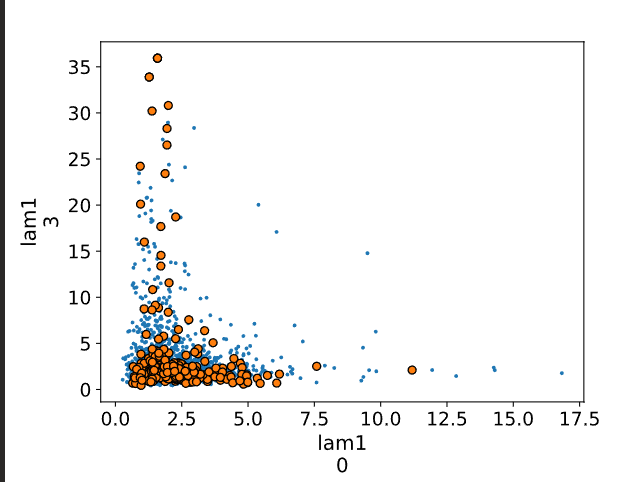
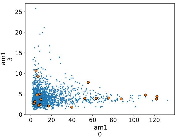
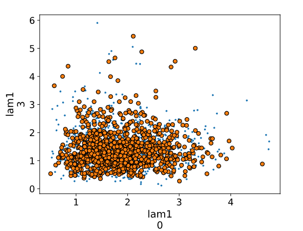
Result:
az.pairplot():
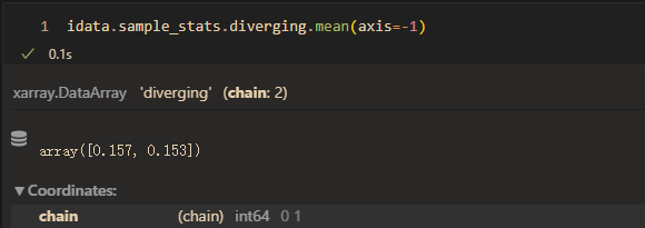
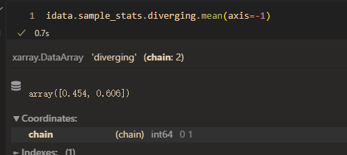
mean(divergent):
Further details about the model are described below, which can also be found in (Cognitive Diagnosis Model).
In educational measurement, cognitive diagnosis models (CDMs) have been used to evaluate the strengths and weaknesses in a particular content domain by identifying the presence or absence of multiple fine-grained attributes (or skills). The presence and absence of attributes are referred to as “mastery” and “non-mastery” respectively. A respondent’s knowledge is represented by a binary vector, referred to as “attribute profile”, to indicate which attributes have been mastered or have not.
The deterministic inputs, noisy “and”" gate (DINA) model (Junker and Sijtsma 2001) is a popular conjunctive CDM, which assumes that a respondent must have mastered all required attributes in order to correctly respond to an item on an assessment.
To estimate respondents’ knowledge of attributes, we need information about which attributes are required for each item. For this, we use a Q-matrix which is an {I×K} matrix where q_{ik}=1 if item I requires attribute k and 0 if not. I is the number of items and K is the number of attributes in the assessment.
A binary latent variable \alpha_{jk} indicates respondent j ’s knowledge of attribute k, where \alpha_{jk}=1 if respondent j has mastered attribute k and 0 if he or she has not. Then, an underlying attribute profile of respondent j, {\alpha_{j}}, is a binary vector of length K that indicates whether or not the respondent has mastered each of the K attributes.
In educational measurement scenarios, measured skills are often correlated and can be modeled using high-order structures to consider the correlations between attributes. Specifically, it is assumed that a high-order ability, represented by \theta_j , influences the probability of mastering multiple attributes as a higher-order factor. Here, \lambda_{0k} represents the intercept, \lambda_{k} represents the slope, and the probability of mastery for the high-order ability \theta_j and attribute \alpha_{k} is connected through a logistic function.
Under the DINA assumption, a respondent can only answer an item correctly if they have mastered all the attributes required by that item.The deterministic element of the DINA model is a latent variable \xi_{ij} that indicates whether or not respondent j has mastered all attributes required for item i:
If respondent j has mastered all attributes required for item i, \xi_{ij}=1; if the respondent has not mastered all of the attributes,\xi_{ij}=0.
The model allows for slipping and guessing defined in terms of conditional probabilities of answering items correctly (Y_{ij}=1) and incorrectly (Y_{ij}=1)
The slip parameter s_i is the probability that respondent j responds incorrectly to item i although he or she has mastered all required attributes. The guess parameter g_i the probability that respondent j responds correctly to item i although he or she has not mastered all the required attributes.
It follows that the probability \pi_{ij} of a correct response of respondent j to item i is
However, due to the presence of latent discrete variables \alpha_{jk} and \xi_{ij}, the NUTS algorithm in numpyro requires the marginalization of these latent discrete variables.
The purpose of the DINA model is to estimate an attribute profile of each respondent. In the framework of latent class models, respondents are viewed as belonging to latent classes that determine the attribute profiles. In this sense,\alpha_{jk} and \xi_{ij} can alternatively be expressed at the level of the latent class subscripted by c. Each possible attribute profile corresponds to a latent class and the corresponding attribute profiles are labeled \alpha_c with elements \alpha_{ck}. The global attribute mastery indicator for respondents in latent class c is defined by
where \alpha_{ck} represents the attribute variable for respondents in latent class c that indicates whether respondents in this class have mastered attribute k {\left(\alpha_{c k}=1\right)} or not {\left(\alpha_{c k}=0\right)}, and q_{i k} represents the binary entry in the Q-matrix for item i and attribute k. Although \xi_{ij} for respondent j s latent, \xi_{ij} is determined and known for each possible attribute profile as a type of characteristic of each latent class.
Then, the probability of a correct response to item i for a respondent in latent class c is represented as follows:
where Y_{ic} is the observed response to item i of a respondent in latent class c.
The marginal probability of a respondent’s observed responses across all items becomes a finite mixture model as follows:
where \boldsymbol y_j is the vector of observed responses y_{i j}(i=1, \ldots, I), \boldsymbol \nu_{c} is the probability of membership in latent class c, and \pi_{ic} is the probability of a correct response to item i by a respondent in latent class c.