Ah, that makes sense. Thank you for your help!
I guess for now I’ll stick to using SVI in Pyro (although I’m looking forward to trying out more models like this in the future if MCMC is developed further!).
Ah, that makes sense. Thank you for your help!
I guess for now I’ll stick to using SVI in Pyro (although I’m looking forward to trying out more models like this in the future if MCMC is developed further!).
I recently implement this model with pyro, however with SVI,
after doing some math, I replace the gauss random walk with a multivariate normal with a special lower triangular matrix, as specified by the following model code:
################## vectorized version
def model_vec(data_vec):
    N = len(data_vec)
    rv_sigma = pyro.sample("rv_sigma", dist.Exponential(torch.tensor(50.)))
    rv_nu = pyro.sample("rv_nu", dist.Exponential(torch.tensor(0.1)))

    # random walks model corresponds to scale_tril of tril of all one matrix
    rv_s = pyro.sample("rv_s", dist.MultivariateNormal(loc=torch.zeros(N)*0.0, scale_tril=torch.ones((N,N)).tril()))
    pyro.sample("obs",
                dist.StudentT(rv_nu, loc=torch.tensor(0.), scale=rv_s.exp()).independent(),
                obs=data_vec)

def guide_vec(data_vec):
    N = len(data_vec)
    ##### params
    p_sigma_1 = pyro.param("p_sigma_1", torch.tensor(0.))
    p_sigma_2 = pyro.param("p_sigma_2", torch.tensor(1.),
                         constraint=constraints.positive)
    p_nu_1 = pyro.param("p_nu_1", torch.tensor(0.))
    p_nu_2 = pyro.param("p_nu_2", torch.tensor(1.),
                        constraint=constraints.positive)


    p_s_loc = pyro.param("p_s_loc", torch.zeros(N))
    p_s_scale = pyro.param("p_s_scale", torch.ones(N),
                        constraint=constraints.positive)


    ##### rvs
    rvq_sigma = pyro.sample("rv_sigma", dist.LogNormal(p_sigma_1, p_sigma_2))
    rvq_nu = pyro.sample("rv_nu", dist.LogNormal(p_nu_1, p_nu_2))
    pyro.sample("rv_s", dist.Normal(p_s_loc, p_s_scale).independent())
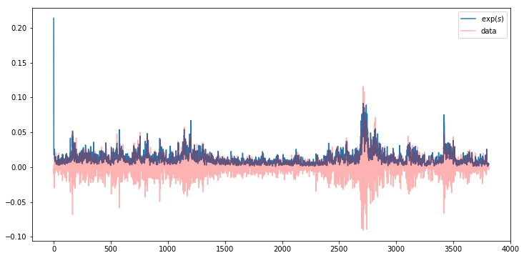
I tried on the sp500 data used by the pymc3 tutorial, however the estimated s is quite unsmooth as shown in the following plot
Any idea of how to improve the inference?
First, I find initialization to be quite important in SVI. You might try initializing p_s_loc to data and p_s_scale to either overestimate or underestimate variance
pyro.param("p_s_loc", torch.abs(data_vec).log1p())  # or similar
pyro.param("p_s_scale", 0.1 * torch.ones(N),
           constraint=constraints.positive)
or maybe
pyro.param("p_s_scale", 10.0 * torch.ones(N),
           constraint=constraints.positive)
Second, I believe your guide can be automatically constructed via
guide = pyro.contrib.autoguide.AutoDiagonalNormal(model)
though you would need to interact with it a bit differently.
Thanks @fritzo for the quick reply. I tried both of the initialization strategy.
However the resulting exp(s) are both unsmooth, as previous result.
I am thinking if fully factorized approximation of s over simplified the problem. In the model, s_t is correlated with s_{t-1}. Is it possible to specify the following approximated posterior in an efficient way in pyro?
p(s) = p(s_0)p(s_1|s_0)p(s_2|s_1)\cdotsp(s_n|s_{n-1})
where each conditional p is a Normal?