If I want to sample from the posterior predictive of a model whose corresponding guide I’ve trained with SVI, I just do the following:
pred = Predictive(model, guide=guide, num_samples=n, return_sites=("t", "y"))
samples = pred(z)
I would like to sample from the same model, but where T is intervened on so that we have do(T = 1). Ideally, that would just be coded as the following:
However, that appears to give me the same samples (assuming I set the same random seed before both), as if Predictive ignores that I’ve used the do-operator. Is it clear what kind of behavior I’d like? If so would you mind pointing me in the right direction for how to do this?
Hi, can you clarify what you mean by “the same samples” and what behavior you expect for the posterior predictive of the intervened site t (since it’s one of the variables in your query)? Do you mean the values for both sites t and y are the same with and without do, or just site t? If both, is there a y site in your guide?
Note that the way do works in Pyro, a t site will appear in your traces but the value used in the model will be the intervened value.
I mean that samples['t'] == do_samples['t'] yields a vector of Trues. And I expected do_samples['t'] to be a vector of 1s (making samples['t'] == do_samples['t']False in all elements where samples['t'] != 1); this check is how I was testing to see if the pyro.do was actually doing something. However, now that I examine samples['y'] and do_samples['y'], they do appear to be different. In case this is useful in the future: I’m just using AutoNormal(model) as my guide (so there is a y site). (EDIT: though, now that I think about it, I do condition on y when training the guide, so I think it isn’t supposed to show up in the guide. I can think about this more later if it becomes important).
This sounds really important, so let me make sure I understand: “a t site will appear in your traces” sounds like it explains why samples['t'] == do_samples['t'] yields a vector of Trues. This means the actual t samples are not constrained to be 1, right (I’m a bit noob at Pyro)? And then “but the value used in the model will be the intervened value” explains why samples['y'] and do_samples['y'] are different, despite the previous sentence.
In other words, the intervened value of t doesn’t affect the samples of t, but it does affect the samples of descendents of t in the graph (e.g. y); does that sound right?
It sounds like your code is working as expected, since there’s no y in your guide.
In other words, the intervened value of t doesn’t affect the samples of t , but it does affect the samples of descendents of t in the graph (e.g. y ); does that sound right?
Yes, that’s right: the value returned from an intervened pyro.sample call is the intervened value. The value you see for the intervened site in the trace has no downstream effect and is typically not meaningful unless you want to observe a different value for that site at prediction time (for example, to compute a query of the form p(y | x, do(t=1), t=0)).
This seemingly strange behavior occurs because Pyro’s do operator follows single world intervention graph semantics, a convenient formalism for computing causal effects of multiple interacting interventions.
Gotcha, I think I mostly understand (enough to use this stuff at least). So everything is actually working then; the behavior for the intervened site was not what I expected, but that doesn’t really matter because the behavior for the y site is what I expect (samples from p(y | do(T = 1))). Thanks!
I guess this could be sufficient motivation to finally read some SWIG literature.
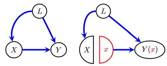
To elaborate a bit more, this figure from the SWIG primer linked above demonstrates conceptually what the do operator in Pyro does to a program represented as a directed graphical model (the new red x node is deterministic and always returns the value x):
This “node-splitting” operation turns out to have two nice computational properties, proved and discussed at length in the main SWIG paper and roughly stated as follows:
One can express any causal effect nonparametrically identifiable via the do-calculus, even those with multiple interventions in the presence of latent variables, as a marginal distribution of a single graphical model obtained via one or more node-splitting operations.
A causal effect such as p(y | do(x)) is nonparametrically identifiable iff the upstream half of the split nodes (i.e. the halves receiving the input edges) are jointly conditionally independent of the post-intervention query node, which can be checked via d-separation in the usual way in the modified graph.
These properties make SWIGs a convenient formalism for causal inference in a PPL like Pyro because node-splitting is easy to implement and all of our usual inferential tools can be applied to the modified model to answer causal queries.
If you want to recover the standard behavior of Pearl’s do-operator, you can simply compose pyro.poutine.do with pyro.poutine.block:
intervened_model = block(do(model, data=data), hide_fn=lambda msg: msg['name'] in data)